Implementing High-Resolution Cloth and Origami Simulations on GPU using XPBD
Clint Wang · May 1, 2026
Introduction and Theory
I recently took a graduate course on physical simulations, taught by the incredibly talented Etienne Vouga. I wanted to apply what I learned, so I built a real-time physical simulation framework for rigid and cloth objects using extended position-based dynamics [XPBD, Macklin et al.].
To evaluate the strengths and limitations of XPBD, I extended a baseline shape-matching PBD cloth simulation with self-collision handling, friction constraints, and collisions against rigid bodies. After discovering the limitations of shape-matching and triangular meshes, I implemented a particle cloth that uses distance constraints. I then created a real-time origami simulation by adding stiff hinge constraints to the cloth model.
The framework is written in Rust that is compiled to WebAssembly (Wasm), and rendered using WebGPU. It can be run directly in the browser or as a headless binary for advanced debugging. A lightweight browser interface exposes key simulation parameters for interactive tuning. The source code is available on GitHub at https://github.com/txst54/wasm-cloth-sim, and a live browser demo is hosted at https://cloth.clintwang.com .
Position-based Dynamics
The baseline cloth simulation uses position-based dynamics (PBD), which can be thought of as a Verlet-like position prediction step, followed by an implicit-style constraint projection. In most implementations, the solver computes a target position, then interpolates between the Verlet predicted position and target position. Let be a stiffness parameter for constraint . The position update is as follows:
More formally, we can say that given a constraint scoring function , the constraint solver computes a per-constraint position delta:
The subscript denotes the iteration index, denotes the constraint index, is the constraint stiffness, and the scaling factor is derived:
Therefore, the issue with PBD is that stiffness depends on the number of constraint projections performed.
In a cloth simulation, the cloth typically has stretching and bending constraints. We refer to the rest position of a cloth as the initial position a cloth started in.
- The stretching constraint defines how individual edges in the cloth interact with respect to the rest position.
- The bending constraint defines how multiple edges in the cloth interact with respect to the rest position.
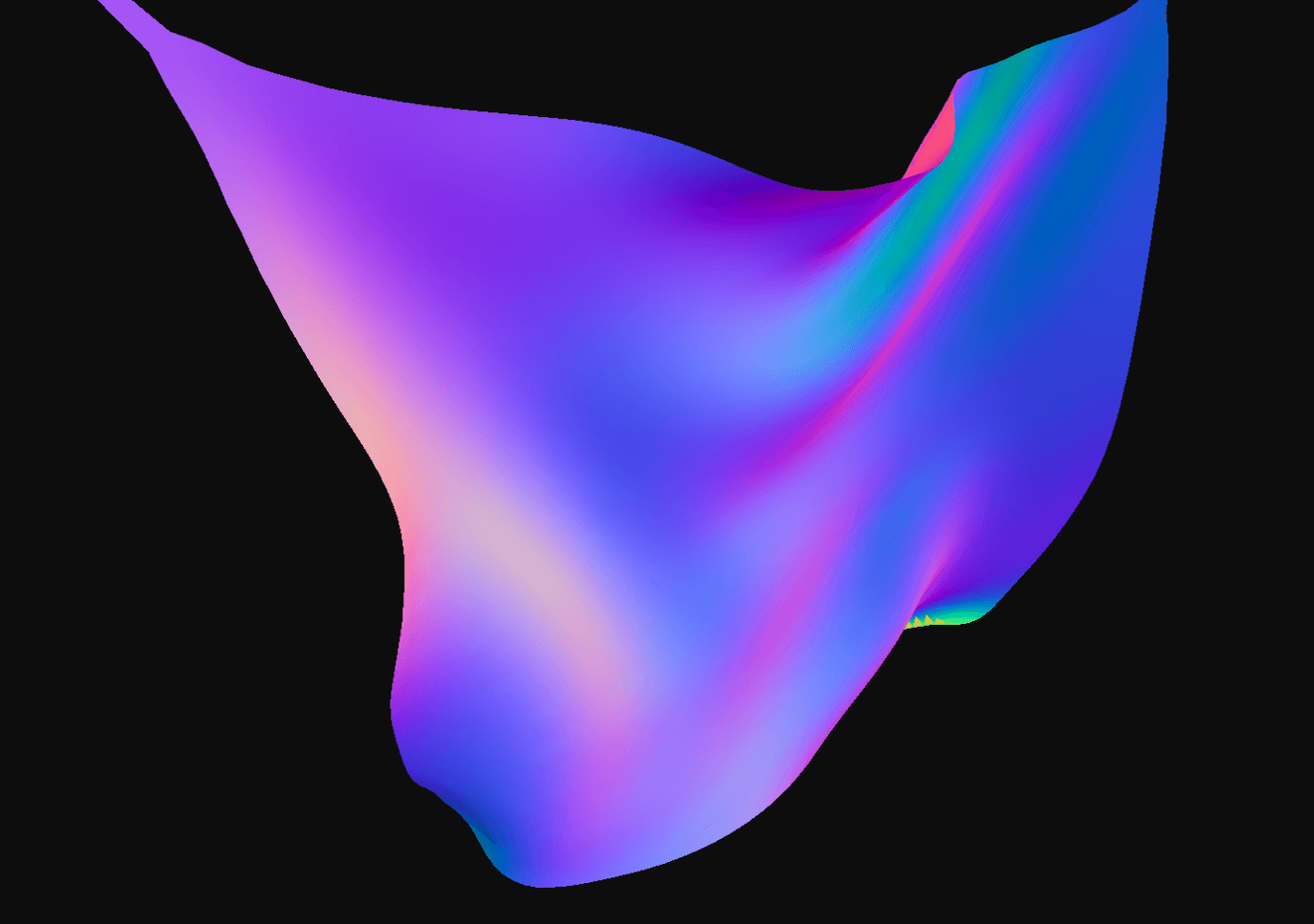
For the PBD cloth simulation stretching and bending constraints, I use shape matching [Meshless Deformations, Muller et al.]. Each triangle in the cloth is constrained to match the corresponding triangle in the rest position via a rotation and a translation. Solving shape-matching is equivalent to solving the orthogonal Procrustes problem, which states that given matrices and , how can we map to using an orthogonal matrix.
The solver computes a target motion directly, which makes it non-trivial to express the constraint as a scoring function C(x). Rather than deriving motion from the gradient of a constraint energy, the method produces the target configuration explicitly. This distinction does not affect the PBD implementation, but becomes problematic in the XPBD formulation, which relies on an explicit constraint function. Additionally, solving the orthogonal Procrustes problem requires an SVD, which is computationally expensive.
Extended Position-based Dynamics
Earlier I mentioned that when using PBD, stiffness depends on the number of iterations. XPBD solves this by introducing compliance (block diagonal compliance matrix corresponding to inverse-stiffness) and a Lagrange multiplier per constraint:
XPBD solves by approximating each constraint as a local linear system and performing a Gauss-Seidel update:
XPBD folds the time step into compliance, defining .
Deriving XPBD
Macklin et al. provide a beautiful derivation of XPBD from Newton's equations of motion, specifically the 2nd law of motion:
If we subject the equation to forces derived from an energy potential , we get equivalently:
We want to discretize . Recall the central difference from high school calculus:
If we differentiate again, we get:
Where superscript refers to the time step index. Plugging into the equation of motion, we get:
Recall from high school physics that elastic potential energy is represented by where is stiffness. Because the constraints represent displacement from natural position, we can reformulate as follows:
Macklin et al. introduce , which represents a block diagonal compliance matrix corresponding to inverse stiffness. Therefore, . We get:
Plugging this back into the equations of motion, we get:
We can define by folding in from the right side of the equation. We can also redefine force elastic using the semantics of a Lagrange multiplier: . Finally, we can define , which is the predicted position computed by Verlet integration. Now we get the following systems of equations:
To solve this coupled nonlinear system, we treat both and as unknowns and define:
so that the system becomes:
However, both equations are nonlinear in due to and , so we solve them using Newton’s method:
The resulting linear system is:
We can then solve and and perform the following update:
Macklin et al. claim that we can set with an error on the order of . They also claim that we can assume since this is true given the initial values and . We get:
By doing a bit of algebra, we can solve for :
Then we can substitute to get the update:
By implementing a Gauss-Seidel solution for the systems of linear equations, we can calculate for a single constraint, then update positions.
XPBD Implementation for Cloth
Because shape-matching does not easily provide a scalar , I chose to keep shape-matching in PBD while creating a new distance constraint option in XPBD:
Users can toggle between the two.
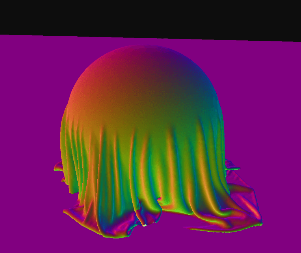
Particle cloth simulation (XPBD distance constraint): High-resolution cloth at 30 FPS, resolution=150, substeps = 1
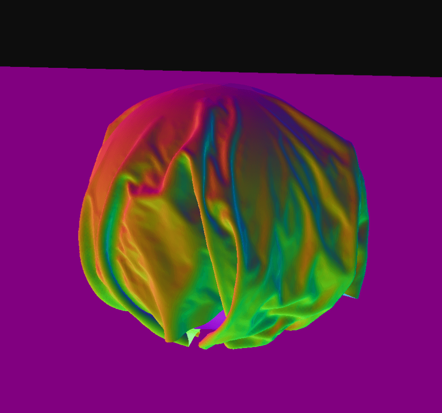
Particle cloth simulation (XPBD distance constraint): High-resolution cloth at 20 FPS, resolution=150, substeps = 10
From the above figures, we see that using more substeps shows less stretching and higher material stiffness.
Self-Collision and Rigid Bodies
For both the triangle and particle cloth collision-detection, I used a spatial hash. The triangle cloth hashes triangles and runs vertex-triangle continuous collision detection (CCD). The particle cloth hashes particles and runs vertex-vertex and sub-stepping.
My implementation of continuous-collision detection predicts collisions along a path by solving for the earliest exact in where intersects any object. I discovered that CCD with triangles is computationally expensive and assumes linear approximation of motion resulting in tunneling.
To solve this, I implemented a particle cloth simulation where collisions are tested betIen vertex particles with a set radius. Since XPBD makes stiffness independent of iteration, I can set the number of iterations at a low number. Macklin et al. state that instead of running 1 timestep and iterations per frame, they obtained a significant improvement by running sub-steps and 1 iteration per frame [Small Steps, Macklin et al.]. By decreasing through sub-stepping, I find that tunneling is virtually eliminated without implementing CCD.
I implemented a stable cloth-cloth friction that blends tangential velocities of contacting points:
The total average velocity remains conserved and the relative velocity always shrinks.
For rigid bodies, I copied the numerical integrators from the rigid body assignment for the base implementation. I implemented a BVH for complex mesh collision and a signed distance field for simple rigid body collisions. I implemented a cloth-rigid body frictional constraint satisfying Coulomb's law:
Where is the frictional coefficient and is the normal Lagrange multiplier.
GPU
To simulate a high-resolution cloth, I found the CPU to be insufficient. Logically, XPBD fits the GPU SIMD model: compute velocity, constraints, and position updates in parallel. However, distance constraints for stretching and bending are co-dependent. Gauss-Seidel updates the positions themselves:
Each update influences neighboring constraints. An alternative is a Jacobi solve that performs the following:
The Jacobi solve updates the initial position produced by Verlet integration. Consequently, the solve takes longer to converge, overshoots, and violates momentum conservation. Therefore, I adopted a hybrid approach. I used greedy graph coloring to iteratively select and concurrently process a subset of independent distance constraints using Gauss-Seidel. Because graph-coloring would yield a large number of colors (small sets) for collision constraints, I handle collision constraints using a parallel Jacobi solve.
Origami
The goal of the origami simulation is to map a mesh of creases on an unfolded sheet of paper to the folded version. Typically, the crease mesh is called a crease pattern and will contain 3 types of edges:
-
Boundary edges represent the edge of the paper and typically form a square.
-
Mountain fold edges represent creases that fold away from you.
-
Valley fold edges represent creases that fold towards you.
I base our implementation on the numerical integrator developed by Ghassei et al. [Origami Simulator, Ghassei et al.]. Ghassei et al. model a force based on a dihedral crease constraint, which naturally maps to an XPBD constraint. I evaluate the constraint on hinge diamonds, which are diamonds that overlay creases. In origami, the dihedral angle is more usefully defined as the angle between the two plane normals, rather than betIen the planes themselves. A flat unfolded hinge diamond will have a dihedral angle of 0 according to our convention. To simulate fold progress, I set , where and is a vector the size of the number of hinges, containing if hinge is a valley fold, or if hinge is a mountain fold.
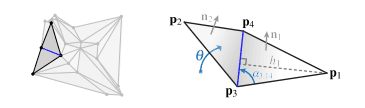
The constraint is rather simple: I also want to know , the gradient of at point . I get:
Following the orientation given by Figure 1, the derivatives for flap vertices are proportional to the normals of their respective triangles: The derivatives for edge vertices are the weighted sum of the flap vertex derivatives.
Origami in PBD versus XPBD
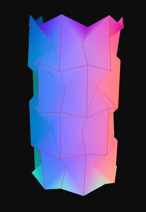
Triangle mesh paper simulation (XPBD shape-matching dihedral angle constraint): Waterbomb tessellation at resolution=1.
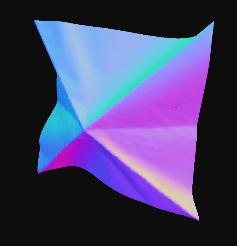
Particle paper simulation (XPBD distance + dihedral angle constraint): Waterbomb base in a high resolution paper, resolution = 64.
One limitation of the particle XPBD paper simulation is that in high resolutions, the distance constraints become slightly unstable. Notice the small bumps in the paper in Figure 4. When I ran simulations in the triangle mesh PBD shape-matching paper simulation, the paper was smooth. This is because shape-matching provides high-fidelity projections onto the rest shapes.
Implementation Details
Architecture
The Rust core of the simulation is located in /rust. All
architecture-specific details (Wasm versus native binary) can be found
in /rust/src/arch. GPU-support is only enabled in the Wasm package,
and the native binary is several commits behind the Wasm package, so
outputs may not look the same.
The Wasm package can be built using
cd rust && wasm-pack build --target web --features gpu. Since Wasm
packages are compiled as a library, the "main" function of the Wasm
package can be found in /rust/src/arch/wasm/harness.rs.
Since the native binary is compiled as a binary, the binary entry point
can be found at /rust/bin/native.rs and wraps
/rust/src/arch/native/harness.rs.
If the GPU compute shaders in particle cloth or particle paper cause
issues, the simulation can be reverted to the serial Gauss-Seidel CPU
implementation by omitting the gpu feature flag. All code relating to
the user interface wrapping the Wasm package is located in /src.
Available Simulations
| URL | Simulation |
|---|---|
/ | Triangle Mesh Cloth Simulation + Rotating BVH Rigid Body |
/paper | Triangle Mesh Paper Simulation |
/particle_cloth | GPU Particle Cloth Simulation + Static SDF Rigid Body |
/particle_paper | GPU Particle Paper Simulation |
I offer 4 simulations located at different sub-URLs. The triangle mesh simulations run shape-matching PBD constraints by default while the particle cloth simulations only run distance XPBD constraints for cloth structure. I have a UI that allows the user to adjust several parameters relating to the simulation. Since scales for parameters may be very small, or on the exponential magnitude, I recommend manually entering numbers into inputs if the sliders do not prove sufficient. Damping and timestep are examples of this.
Available Crease Patterns
| Crease Pattern | Description |
|---|---|
line.cp | A single vertical crease |
lines.cp | Two vertical creases |
waterbomb.cp | A traditional origami base |
miura_ori.cp | A classic and easy to fold origami tessellation |
waterbomb_tess.cp | A classic and harder to fold origami tessellation |
hex_torso.cp | Modern origami "hex-pleat" model. Designed by Clint. |
Table: Available crease patterns for paper simulation